Diffusion

A review of diffusion: 1. law of diffusion: Fick’s 1^st law, Fick’s 2^nd law

1^st law J=-D∂c/∂x, “-“決定濃→淡方向; ∂c/∂x: concentration gradient

J: atoms/cm²sec (flux), x: cm, c: atom/cm³, D: cm²/sec

*single phase: 只考慮單純系統,若有共析相等產生,則1^st law須修正

Atomic meaning of D (p.37, TIM): considering two adjacent atomic planes containing n₁ and n₂ solute atoms per unit area and separated by a distance α.

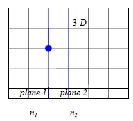
No. of solute atoms jumping from plane 1 to plane 2 per unit area in time δt, Γδtn₁/6-Γδtn₂/6=Jδt,

: jumping frequency(an atom jumping to nearest adjacent site)與振動頻率有關

if one dimension: 1/6 →1/2

Γ=rexp(-Ei/kT)exp(Δs/k), r: 可供最大利用的空位位置數

Γn₁/6-Γn₂/6=J, but n₁/α=c₁ and n₂/α=c₂ where n: atom/area, α: jumping distance spacing between plane 1 and 2. → J=Γα(c₁-c₂)/6

On a macroscopic scale c varies continuously with x: c₂= c₁+(∂c/∂x)_tα

thus J=-Γα²(∂c/∂x)_t/6↔J=-D(∂c/∂x)_t, i.e. D=Γα²/6 for 3-D

Fick’s 2^nd law (non-steady state: c may change with time)

∂c/∂t=∂(D∂c/∂x)/∂x if D is not a function of c → ∂c/∂t=D∂²c/∂x², D=constant

Derivation of Fick’s 2^nd law assuming Fick’s 1^stlaw is valid

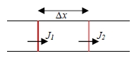
No. of atom of solute entering element ∆x in time δt

J₁Aδt-J₂Aδt=AΔxδc → J₁-J₂=Δx(∂c/∂t)…(1)

but J varies continuously with x, therefore J₂=J₁+Δx(∂J/∂x)…(2)

combining (1) & (2) → ∂c/∂t=-∂J/∂x, but J=-D∂c/∂x and → ∂c/∂t=∂(D∂c/∂x)/∂x

→ ∂c/∂t=D∂²c/∂x²=D²c

Solution to Fick’s 2^nd law

ex-1 Sinusoidal concentration gradient, c(x,0)=c+βsin(πx/l) (initial condition)

c(x,y)=c+βsin(πx/l)exp(-Dtπ²/l²)=c+βsin(πx/l)exp(-t/τ)

where τ=l²/Dπ²=relaxation time=time for a 63.2% decrease in amplitude at t=τ

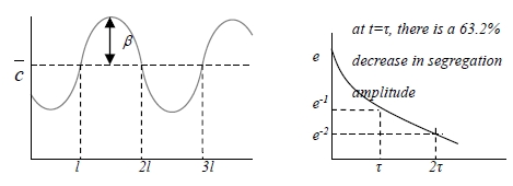
*作homogenization事實上不能完全達到,須定一極限 t=l²/Dπ² effective diffusion time, on other case t=l²/4D effective diffusion time effective diffusion distance x=(π²Dt)^1/2, on other case x=(4Dt)^1/2

ex. 2 thin film solution

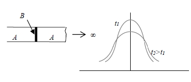
c→0 for x≠0, c→ for x=0 ∫_₋∞^∞c(x,t)dx=α

In practice, a 5cm bar serve as an infinite bar c(x,t)=[α/2(πDt)^1/2]e^-x²/4Dt

2. Atomic theory of diffusion

a. Random nature of diffusion (DIS p.47-57)

p: probability that atom jumps to right(1-p: left)

n: total No. of jumps=t, k: No. of jumps to right, n-k: No. of jumps to left

i: final position of atom=k-(n-k)=2k-n

x=ia : final distance from origin where a spacing between atoms

Probability that an atom will make k jumps to right in n jumps and end up at i position. p(i)=p(k)=(n!/[k!(n-k)!])p^ₖ(1-p)^ₙ⁻^ₖ for large n

p(i)=p(k)≈(1/[2πnp(1-p)]^1/2)exp[-½{(k-np)/[np(1-p)]}²]

for random walk in the absence of p=½ → p(i)=[2/πn]^1/2exp[-½{(k-n/2)/(n/4)^1/2}²]

but k=n/2+i/2 and → p(i)=[2/πn]^1/2exp[-½{i/(n)^1/2}²]=[2/πn]^1/2exp[-i²/2n]

but x=ia and n=t, where : jumping frequency at t

→ p(i)=[2/πt]^1/2exp[-x²/2a²t] for diffusion in one dimension, D=Γa²/2

p(i)=p(x,t)=[2/πt]^1/2exp[-x²/2a²t]=a[2∙½/½πa²t]^1/2exp[-½(½x²/½a²t)]

p(x,t)=a/(πDt)^1/2exp[-x²/4Dt)] : the probability of finding a B atom at x and t.

p(x,t) is equal to the atomic fraction of B atoms, X_B at x and t.

X_B(x,t)=a/(πDt)^1/2exp[-x²/4Dt)] atoms per unit length in 1-D problem corresponds to atoms per unit volume in 3-D problem.

also X_B=N_B/N where N_B= No. of B atoms/area and N= No. of atoms/area

N_B (x,t)/a=N/(πDt)^1/2exp[-x²/4Dt)] but N=α and N_B/a=c_B → c_B (x,t)=α/(πDt)^1/2exp[-x²/4Dt)]

b. Mechanisms (DIS p.43-46): Interstitial diffusion—C, H, N in Fe, Vacancy diffusion—all substitutional solid solutions

c. Vacancy Diffusion(DIS P.55-57)

equilibrium concentration of point defects N_v^e=e^-∆Gᵥ/kT

N_v: molar fraction of vacancy, N_v^e: probability that a vacancy will exist a certain lattice site, ∆G_v: ∆G_v =∆H_v -T∆S_v ,free energy of formation a vacancy

d. Atomic meaning of D for a simple cubic structure: D=Γα²/6

for interstitial mechanism: D=Γα²/6 , Γ=vexp(-ΔG_m/kT) → Dᵢ=(α²v/6)exp(-ΔG_m/kT)

for vacancy mechanism: Γ=ωpᵥ=ωN_v^e=ωe^-∆Gᵥ/kT

therefore D=Γα²/6=α²ωe^-∆Gᵥ/kT/6=α²ve^-ΔGm/kTe^-∆Gᵥ/kT/6

→ Dₛ=D₀e^-Q/kT, Q: activation energy for diffusion

D_s的energy barrier比D_i多∆G_v這一項→ D_i > D_s

e. experimental techniques for measuring D_v

radioactive tracer method

a. plate tracer on surface of semi-infinite solid

b. diffuse trace at some temperature

c. measure tracer activity as a function of depth of penetration

d. plot log of activity vs. the square of the depth

e. slope of graph is 1/4Dt

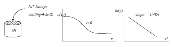
the solution of above core: c (x,t)=α/2(πDt)^1/2exp[-x²/4Dt)]

lnc (x,t)=ln[α/2(πDt)^1/2]-x²/4Dt, c(x,t)  radioactivity counts

Kirkendall effect(diffusion in a concentration gradient) p.115 DIS

不是由grain boundary或lattice point擴散vacancy,是藉dislocation來消除、減少,維持平衡濃度

B. High diffusion paths(chapter 6 DIS)

Region in crystalline solids where the diffusion rate is faster than that in the crystal lattice itself.

1. type of high diffusion path: dislocation, grain boundary, free surface提供atom克服∆G_m的能量

2. experimental observation:

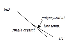
D=D₀e^-Q/kT

a. higher than expected diffusivity in polycrystal at low temperature.

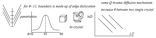
b. tilt boundary diffusivity

3. Mechanism

a. dislocation: stress field—high vacancy concentration, higher diffusivity

N_v=e^-Q/kT vs. N_vd=e^{(-Q/RT+σV/RT)} N_vd >N_v

b. grain boundary diffusion: low angle boundary same as dislocation, high angle boundary similar to low angle but cannot mathematically described.

c. free surface: unknown possibly ledges

4. Theories

a. Grain boundary diffusion (Fisher’s model)

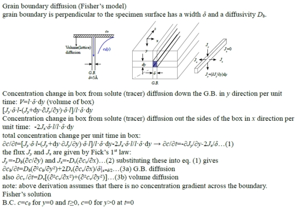
grain boundary is perpendicular to the specimen surface has a width δ and a diffusivity D_b.

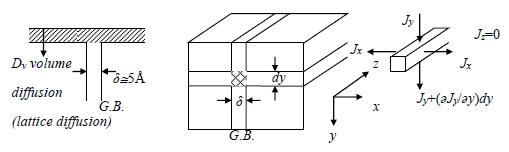
Concentration change in box from solute (tracer) diffusion down the G.B. in y direction per unit time: V=l·δ·dy (volume of box)

[J_y∙δ∙l-(J_y+dy∙∂J_y/∂y)∙δ∙l]/l·δ·dy

Concentration change in box from solute (tracer) diffusion out the sides of the box in x direction per unit time: -2J_x∙δ∙l/l·δ·dy

total concentration change per unit time in box:

∂c/∂t=[J_y∙δ∙l-(J_y+dy∙∂J_y/∂y)∙δ∙l]/l·δ·dy-2J_x∙δ∙l/l·δ·dy → ∂c/∂t=-∂J_y/∂y-2J_x/δ…(1)

the flux J_y and J_x are given by Fick’s 1^st law:

J_y =-D_b(∂c/∂y) and J_x=-D_v(∂c_v/∂x)…(2) substituting these into eq. (1) gives

∂c_b/∂t=D_b(∂²c_b/∂y²)+2D_v(∂c_v/∂x)/δ|_x=δ/2…(3a) G.B. diffusion

also ∂c_v /∂t=D_v[(∂²c_v/∂x²)+(∂²c_v/∂y²)]…(3b) volume diffusion

note: above derivation assumes that there is no concentration gradient across the boundary.

Fisher’s solution

B.C. c=c₀ for y=0 and t≥0, c=0 for y>0 at t=0

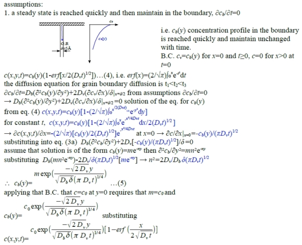
assumptions:

1. a steady state is reached quickly and then maintain in the boundary, ∂c_b/∂t=0

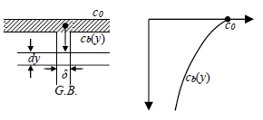
i.e. c_b(y) concentration profile in the boundary is reached quickly and maintain unchanged with time.

B.C. c_v=c_b(y) for x=0 and t≥0, c=0 for x>0 at t=0

c(x,y,t)=c_b(y)(1-erf[x/2(D_vt)^1/2])…(4), i.e. erf(x)=(2/√π)∫₀^xe^-t²dt

the diffusion equation for grain boundary diffusion is t₁23

∂c_b/∂t=D_b(∂²c_b(y)/∂y²)+2D_v(∂c_v/∂x)/δ|_x=δ/2 from assumptions ∂c_b/∂t=0

→ D_b(∂²c_b(y)/∂y²)+2D_v(∂c_v/∂x)/δ|_x=δ/2 =0 solution of the eq. for c_b(y)

from eq. (4) c(x,y,t)=c_b(y)[1-(2/√π)∫₀^x/2(Dvt)1/2 e^-y²dy]

for constant t, c(x,y,t)=c_b(y)[1-(2/√π)∫₀^xe^-x²/4Dvtdx/2(D_vt)^1/2

→ ∂c(x,y,t)/∂x=-(2/√π)[c_b(y)/2(D_vt)^1/2]e^-x²/4Dvt at x=0 → ∂c/∂x|_x=0=-c_b(y)/(πD_vt)^1/2

substituting into eq. (3a) D_b(∂²c_b/∂y²)+2D_v[-c_b(y)/(πD_vt)^1/2]/δ =0

assume that solution is of the form c_b(y)=me^-ny then ∂²c_b/∂y²=mn²e^-ny

substituting D_b(mn²e^-ny)-2D_v/δ(πD_vt)^1/2[me^-ny] → n²=2D_v/D_b δ(πD_vt)^1/2

 c_b(y)= …(5)

applying that B.C. that c=c₀ at y=0 requires that m=c₀ and

c_b(y)= substituting

c(x,y,t)=

擴散: 原子遷移的微觀過程及其引起的宏觀現象,例如: 相變化,氧化, 脫碳, 滲碳, 燒結, 均勻化,潛變.

1^st Ficks law:原子從高濃度向低濃度區域流動

J=-D(∂c/∂x), 單位時間通過某一截面的量, J與∂c/∂x的方向相反, D:比例係數

J, D, ∂c/∂x可以是常數,也可以是變數.

如圖: ⸪ ∂c/∂x|ₓ₁>∂c/∂x|ₓ₁₊_dₓ ⸫ J(x₁)>J(x₁+dx)

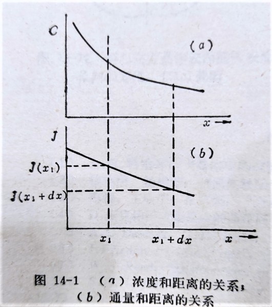
dx的體積中濃度變化速率, ∂c/∂t → ∂c/∂t|ₓ₁∙dx=J(x₁)-J(x₁+dx)...(1)

if dx→0, J(x₁+dx)=J(x₁)+∂J/∂x|ₓ₁∙dx...(2), 比較(1)(2)

→ ∂c/∂t=-∂J/∂x=-∂/∂x(-D(∂c/∂x)), ∂c/∂t=D∂²c/∂x²...2^nd Ficks law

擴散方程式的應用

(i)穩定擴散, steady state, ∂c/∂t=0 不隨時間改變, 因此∂J/∂x=0, J=A₀

ex. 測定1000℃退火γ鐵中碳的擴散係數D, 半徑r的薄壁鐵管,管外保持滲碳濃度c₁, 管內保持脫碳濃度c₂;c₁>c₂, 經過長時間,管壁中的濃度不隨時間變化, 即∂c/∂t=0 → q/t=B₀ q: 流進或流出的總碳量, ⸫ J=q/(2πrLt)=-D∂c/∂r

→ q=-D(2πLt)∙∂c/∂lnr, c對lnr作圖求斜率可得D, 由於 q/t=B₀為一常數,若D不隨濃度改變, 那麼∂c/∂lnr也是常數, 作圖會得一直線!

但實驗指出高濃度區域斜率較小,所以D較大;反之低濃度區域斜率大,因此D較小,可見D為濃度的函數

(ii) 非穩定擴散

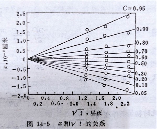
case I: D為常數的半無限長一維擴散, ex. 滲碳, 含碳量c₀的鋼件,置於950℃的滲碳氣氛中,表面維持cₛ的碳濃度(cₛ>c₀)

∂c/∂t=D∂²c/∂x² 初始條件c(x,0)=c₀...(1), c(0,t)=cₛ...(2)

→ c(x,t)=c₀+(cₛ-c₀)[1-erf(x/2√Dt)]

只要x>>2√Dt, 視為無限長一維擴散; 我們發現無論D是常數或是濃度的函數, → x√t, 告訴我們原子遷移的特徵,類似布朗運動中質點隨機行走的方式,但沒有氣、液相中的質點行走那麼自由!

D與溫度的關係: D=D₀exp(-Q/RT)

case II: D隨濃度而變的全無限長一維擴散, ex. Cu-CuZn擴散偶

∂c/∂t=∂/∂x(D(∂c/∂x)) 初始條件c(x>0,0)=c₀...(1), c(x<0,0)=0...(2) span="">

令η=x/2√t, ∂η=∂x/2√t

∂c/∂t=(∂c/∂η)∙(∂η/∂t)=-(x/4t^3/2)∙(∂c/∂η)...(a), ∂c/∂x=(∂c/∂η)∙(∂η/∂x)=1/2√t∙(∂c/∂η)...(b)

(a)(b)代入原式, -(x/4t^3/2)∙(∂c/∂η)=∂/(2√t∂η)[(D/2√t)∙(∂c/∂η)]

→ -(x/4t^3/2)∙(∂c/∂η)=1/4t[∂/∂η(D(∂c/∂η))]→ (x/√t)∙(dc/dη)=d/dη(D(dc/dη))

→ -2η(dc/dη)=d/dη(D(dc/dη)) 初始條件c(+∞,0)=c₀...(1), c(-∞,0)=0...(2)

求c₁時的D_c₁(0<c₁<c₀), 對η積分→ ∫₀^с¹-2ηdc=D(dc/dη)|₀^с¹=D(dc/dη)|_c₁-D(dc/dη)|₀

⸪ dη=dx/2√t, D(dc/dη)=2D√t(dc/dx), 當c=0時, dc/dx=0|ₓ₌₀ ⸫ ∫₀^с¹-2ηdc=D(dc/dη)|_c₁

→ -2∫₀^с¹(x/2√t)dc=2D_c₁√t(dc/dx)|_c₁→ D_c₁=-(1/2t)(dx/dc)|_c₁∙∫₀^с¹xdc

所以在c-x曲線上求得(dx/dc)|_c₁斜率和∫₀^с¹xdc積分,即可得D_c₁

但是∫₀^с¹xdc, x的零點在哪裡? x=0的截面稱作俣野面Matano interface, 與起初的接合面不一定重合, 如何確定俣野面?

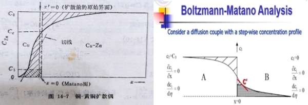
前述當c=0時, dc/dx=0|ₓ₌₀, 同理當c=c₀ 時, (dc/dx)|_c₁=0 ⸫ D(dc/dη)|₀^с₀=0

因此∫₀^с₀ηdc=0=(1/2√t)∫₀^с₀xdc→ ∫₀^с₀xdc=0 為了滿足此條件,俣野面兩邊的積分面積必須相等,若取俣野面上的濃度cₘ,

→ ∫₀^сₘxdc=-2t∙D_cₘ∙(dc/dx)|_c₁=2tJ_cₘ 且 ∫₀^сₘxdc+∫_сₘ^с₀xdc=0

此俣野面的流量與積分面積成正比,流進和流出的量相等,淨流量為零

(iii)均勻化, ex. 均質化處理

假設初始濃度分布沿某一方向呈周期性變化, c(x)=c₀+cₘcos(πx/l)

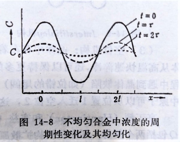
若D不隨濃度改變, c(x,t)=c₀+cₘcos(πx/l)exp(-π²Dt/l²), τ=l²/π²D

→ c(x,t)=c₀+cₘcos(πx/l)exp(-t/τ), τ有關均勻化速度的快慢, 減少τ可加速均勻化,方法有(1)升溫使D增加, (2)降低l, 使晶粒或相尺寸縮小(細化)

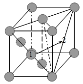
擴散的微觀機構: (1)交換, (2)間隙, (3)空位

(1)交換指兩相鄰原子對調,但會使晶格發生形變,理論和實際上都不可行

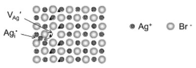
(2)間隙是指間隙原子從一個間隙遷移到鄰近的間隙位置,適用於間隙固溶體, ex. 碳在α鐵或γ鐵的八面體間隙(octahedron);另一種是interstitialcy機構,如Ag 離子在AgBr晶格中遷移

(3)空位:在晶體中每個溫度都有一定的平衡空位濃度,如果從高溫急冷,還有更多的空位,只是存在的時間有限,空位對原子遷移有很重要的作用

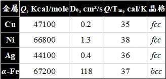
ex. 銅的自擴散,實驗求得活化能,Q=47.1 Kcal/mole,發現空位擴散機構的計算值比較接近

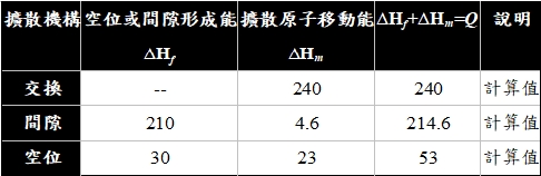
若是稀薄的間隙固溶體,由於鄰近的間隙位置往往是空的(∆H_f=0),Q值也比較小

原子遷移與擴散係數

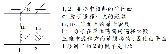
如上圖,以統計觀點考慮δt時間內,由平面1移到平面2的原子數=n₁Γδt/6;同理, 由平面2移到平面1的原子數=n₂Γδt/6,所以由平面1移到平面2的淨通量

J=(n₁-n₂)Γ/6, 將面密度換算成濃度, n₁/α=c₁, n₂/α=c₂代入

J=(c₁-c₂)αΓ/6, ⸪ ∂c/∂x=(c₂-c₁)/α → J=(-α²Γ/6)(∂c/∂x) ⸫ D=α²Γ/6

*前提是各方向在隨機下,原子遷移的距離和頻率必須相同,否則會有異向性,不適用於非立方晶格

擴散係數取決於遷移距離α 和遷移頻率Γ, α 有關於晶格類型和晶格常數;Γ會受溫度、溶質和溶劑原子不同的差異而影響,但無法理論計算,只能近似設想:

Γ=ZPᵥω, Z: 擴散原子的配位數, Pᵥ:鄰近位置是空位的機率, ω:遷入空位的頻率

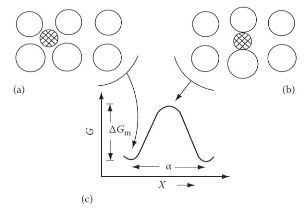
考慮稀薄的fcc間隙固溶體中間隙原子的擴散,八面體間隙的配位數Z=12, 由於稀薄的關係,可視間隙位置都是空位(Pᵥ=1), ω 可表示為 ω=vexp(-∆Gₘ/RT)

i.e. v:振動頻率, ∆Gₘ:遷移的自由能障,當溫度上升, ω就會增大

fcc的α=√2a₀/2, a₀:晶格常數, 因此間隙原子的擴散係數可表述成:

D=α²Γ/6=α²ZPᵥω/6=α²ZPᵥvexp(-∆Gₘ/RT)/6=(√2a₀/2)²∙12∙vexp(-∆Gₘ/RT)/6

=a₀²vexp(-∆Gₘ/RT) ⸪ ∆Gₘ=∆Hₘ-T∆Sₘ代入上式

D=a₀²vexp(-∆Gₘ/RT)=a₀²vexp(-∆Sₘ/R)exp(-∆Hₘ/RT) vs. D=D₀exp(-Q/RT)

→ D₀=a₀²vexp(-∆Sₘ/R), Q=∆Hₘ

同理, bcc 結構的間隙固溶體,間隙原子的擴散係數:

D=α²ZPᵥvexp(-∆Gₘ/RT)/6=(a₀/2)²∙4∙vexp(-∆Gₘ/RT)/6=a₀²vexp(-∆Gₘ/RT)/6

D=[a₀²vexp(-∆Sₘ/R)/6]exp(-∆Hₘ/RT)

純金屬的空位機構自擴散: 由於純金屬是均勻的,不存在濃度梯度,因此用同位素做退火擴散,測量同位素的擴散深度, 其自擴散係數定義為: 

對於fcc結構的純金屬,需要補充討論的是『鄰近位置是空位的機率』Pᵥ,Pᵥ 等於平衡空位濃度Nᵥ, Nᵥ=exp(-∆G_f/RT)=exp(∆S_f/R)exp(-∆H_f/RT)

所以擴散係數可表述成:

D=α²ZPᵥω/6=(α²Zv/6)exp(-∆G_f/RT)exp(-∆Gₘ/RT)

={α²Zvexp[(∆S_f+∆Sₘ)/R]/6}∙exp[-(∆H_f+∆Hₘ)/RT]

=a₀²vexp[(∆S_f+∆Sₘ)/R]∙exp[-(∆H_f+∆Hₘ)/RT] i.e. α=√2a₀/2, Z=12

→ D₀= α²Zvexp[(∆S_f+∆Sₘ)/R]/6, Q=∆H_f+∆Hₘ

同理, bcc 結構的擴散係數, D=a₀²vexp[(∆S_f+∆Sₘ)/R]∙exp[-(∆H_f+∆Hₘ)/RT]

i.e. α=√3a₀/2, Z=8

置換型substitutional雜質在純金屬中的擴散: 與自擴散的差異在於雜質原子和純金屬原子不同,影響到Pᵥ和ω的表現在活化能有何不同? 就價電子或尺寸效應來考慮

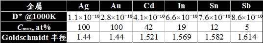
ex. Cd* diffusion in Ag, Cd有2個價電子,比Ag多1個,所以Cd的價電子,1個是自由的,1個束縛在Cd⁺⁺附近,產生被屏蔽的靜電場: (Ze/r)e^-qr i.e. Z:溶質溶劑原子價差, q:屏蔽係數

假定Cd⁺⁺鄰近位置移去一個Ag⁺,形成空位時,空位電荷為-e, 在靜電場中,空位被吸引,位能下降V(r₀)=-(Ze²/r₀)e^-qr₀ 也就是Cd⁺⁺鄰近空位的形成能∆H_f(Cd)=∆H_f(Ag)+V(r₀)比較小

另外,Cd⁺⁺與空位相互作用,使∆Hₘ降低,即∆Hₘ(Cd)=∆Hₘ(Ag)+V(r₀),因此其活化能得

∆H(Cd)=∆H(Ag)+2V(r₀) 同理,對於三價的In: ∆H(In)=∆H(Ag)+4V(r₀)

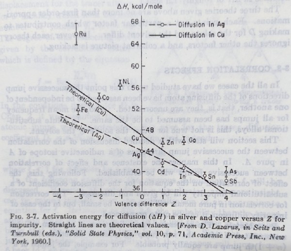
Cd, In, Sn, Sb, Ru在銀中的自擴散活化能,隨原子序的增加,溶質自擴散活化能下降,使自擴散係數增大; 若以尺寸效應解釋,大小差異使應變能增加,活化能減小,不過應變能如何影響∆H_f和∆Hₘ未有定論

相關效應

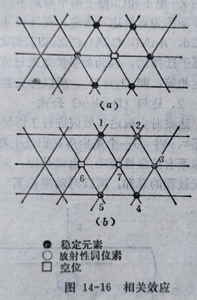
擴散原子遷移的方向是隨機的,n次遷移與第n+1次遷移在各個方向上有相等的 機率,空位擴散也是如此!(如圖a)

Kirkenall效應: Cu-α黃銅(70-30)置換固溶體擴散實驗

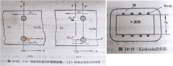
發現: (1)Mo棒向黃銅測移動, (2)Zn原子的尺寸大於Cu,但移動的距離比尺寸差距大很多, (3)結論: 通過Mo棒的流量, J_Zn>J_Cu, D_Zn>D_Cu;因為D₁≠D₂造成Mo棒標記移動,稱作Kirkenall效應,支持了空位機制做擴散中的角色

對移動座標y-x,永遠只看到擴散性流動: J_Zn=-D_Zn(∂c_Zn/∂x), J_cu=-D_Cu(∂c_Cu/∂x)

對固定座標y-x,不只擴散性流動,還有標記移動的整體性流動:

J_Zn=-D_Zn(∂c_Zn/∂x)+c_Znv, J_cu=-D_Cu(∂c_Cu/∂x)+c_Cuv i.e. v: 標記移動速度

以D₁, D₂代替D_Zn, D_Cu 變成一般性討論:

由物質守恆的連續性原則∂c/∂t=-∂J/∂x, 將上述兩式改寫

∂c₁/∂t=∂[D₁(∂c₁/∂x)-c₁v]/∂x...(a), ∂c₂/∂t=∂[D₂(∂c₂/∂x)-c₂v]/∂x...(b) i.e. c₁+c₂=c

(a)+(b), ∂c/∂t=∂[D₁(∂c₁/∂x)+D₂(∂c₂/∂x)-cv]/∂x

令∂c/∂t=0, 意即單位體積內的原子數不隨時而變化

→ ∂[D₁(∂c₁/∂x)+D₂(∂c₂/∂x)-cv]/∂x=0, D₁(∂c₁/∂x)+D₂(∂c₂/∂x)-cv=I₀

I₀=? 設想x→∞, ∂c₁/∂x=∂c₂/∂x=0 且 v_∞=0 ⸫I₀=0→ v=[D₁(∂c₁/∂x)+D₂(∂c₂/∂x)]/c...(c)

將(c)代入(a), ∂c₁/∂t=∂[D₁(∂c₁/∂x)-c₁[D₁(∂c₁/∂x)+D₂(∂c₂/∂x)]/c]/∂x

由濃度換成莫耳分數, N₁=c₁/c, N₂=c₂/c and N₁+N₂=1 → ∂N₁/∂x=-∂N₂/∂x

上式同除c → ∂N₁/∂t=∂[D₁(∂N₁/∂x)-N₁D₁(∂N₁/∂x)-N₁D₂(∂N₂/∂x)]/∂x

=∂[N₂D₁(∂N₁/∂x)-N₁D₂(∂N₂/∂x)]/∂x=∂[N₂D₁(∂N₁/∂x)+N₁D₂(∂N₁/∂x)]/∂x

→ ∂N₁/∂t=∂[(N₂D₁+N₁D₂)(∂N₁/∂x)]/∂x define Ð=N₂D₁+N₁D₂

∂N₁/∂t=∂[Ð(∂N₁/∂x)]/∂x

在Cu-α黃銅(70-30)擴散實驗中,如果N_Zn→0, Ð≈D_Zn

因此Ficks law需包括Kirkendall效應加到流量總和裡: J₁=-Ð∂c₁/∂x, J₂=-Ð∂c₂/∂x